Hessian analysis with JAX: a platform-agnostic, high-performance approach

July 31, 2025

In mechanistic interpretability research, we often want to analyze the Hessian of the loss function (for example, by computing its eigenspectrum). Ideally, we would want our Hessian analysis code to work seamlessly for all models irrespective of architecture or training platform (e.g. PyTorch, tensorflow, flax, etc.). However, this is hard to achieve because of platform-specific interfaces for accessing information about the model (e.g. datasets, parameters, and functions). As a result, we end up tightly coupling our analysis code with the training platform, forcing unnecessary re-writes when switching platforms.

The goal of this post is to present a simple, JAX-based framework to address the above difficulty. This framework will help us:

make the core numerical code platform-independent, allowing it to be optimized separately and used across models/platforms.
formalize the changes needed to peripheral code when switching platforms, minimizing the possibility of errors.
disentangle model training from Hessian analysis, facilitating the analysis of pre-trained models.

(I am currently working on a SPAR project where we have used the above framework quite successfully.)

NOTE: For analyzing a model, it is not necessary to train it ourselves as long as we have access to certain defining attributes of the model (details in post).

NOTE: There are several reasons for choosing JAX for this task - performance, flexibility, math-like flavor, numpy-like interface, and the powerful Pytree abstraction for parameter handling (more on each of these in a future post).

NOTE: Even if you don’t anticipate working across multiple platforms, you may still want to consider this framework for the above reasons.

NOTE: This post assumes the reader is familiar with eigsh and how it can be used to compute the Hessian eigenspectrum via Hessian-vector products. (As a refresher, I recommend reading this post upto, but excluding, the implementation which is very Pytorch specific.)

NOTE: The code presented here is written for simplicity and clarity, not for compute or memory efficiency. I will try to point out obvious optimizations where possible.

NOTE: The code presented here runs on a single CPU/GPU/TPU. While JAX provides excellent primitives for distributed computations, these are out of scope for this post.

NOTE: This post can be run as a colab notebook here.

A two-part framework

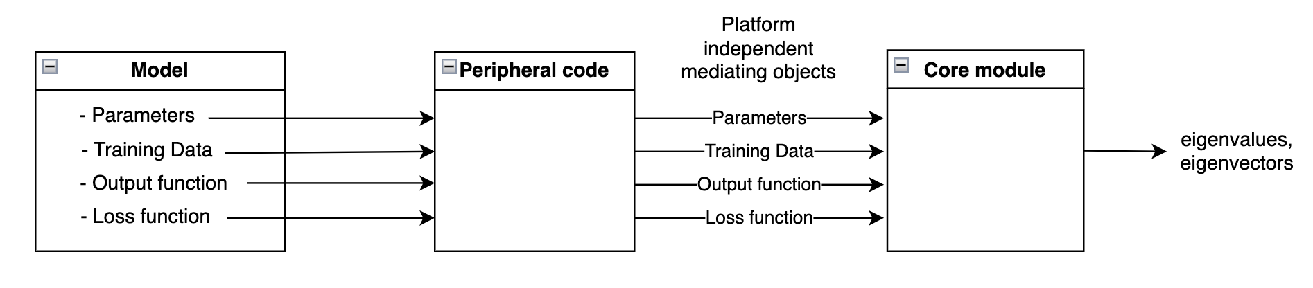
The proposed framework has two parts:

a core module that contains the numerical code to compute the hessian eigenspectrum
a set of mediating objects that implement a standard interface for the core module (to interact with different platforms).

In essence, the mediating objects are a platform-independent representations of the four defining attributes of a model:

model parameters
training data
output function
loss function

For each new model we want to analyze, we first generate the mediating objects and then pass them on to the (platform-agnostic) core module for eigenspectrum computation.

A key observation behind this framework is that numerical code (e.g. computing the eigenspectrum) requires careful memory / compute optimizations and precision handling. As a result, such code should be independent of, and shared across all models/platforms. In particular, this code should not require changes when switching models/platforms. And, while some code changes are inevitable, these changes should be few and limited to parts that are easier to implement and test.

A PyTorch Example

Let’s start by looking at a concrete example. Suppose we want to compute the eigenspectrum of a toy PyTorch MLP model. For this example, we will train the model ourselves.

import torch
import torch.nn as nn
import torch.optim as optim
import numpy as np

# Dataset
X_np = np.array([[1., 2.], [3., 4.]])   # shape (2, 2)
Y_np = np.array([5., 6.])              # shape (2,)

# Convert to PyTorch tensors
X = torch.tensor(X_np, dtype=torch.float32)            # (2, 2)
Y = torch.tensor(Y_np, dtype=torch.float32).unsqueeze(1)  # (2, 1)

# Define MLP with identity activations
class IdentityMLP(nn.Module):
    def __init__(self):
        super().__init__()
        self.fc1 = nn.Linear(2, 2, bias=True)  # Hidden: 2x2
        self.fc2 = nn.Linear(2, 1, bias=True)  # Output: 2x1

    def forward(self, x):
        x = self.fc1(x)  # Identity activation (no-op)
        x = self.fc2(x)  # Identity activation (no-op)
        return x

# Initialize model, loss, and optimizer
torch.manual_seed(0)

model = IdentityMLP()
criterion = nn.MSELoss()
optimizer = optim.SGD(model.parameters(), lr=0.01)

# Training loop (2 epochs, full batch)
for epoch in range(10):
    optimizer.zero_grad()
    output = model(X)       # Forward pass
    loss = criterion(output, Y)  # Compute loss
    loss.backward()         # Backpropagation
    optimizer.step()        # Gradient update
    print(f"Epoch {epoch+1}, Loss: {loss.item():.4f}")

Epoch 1, Loss: 50.2097
Epoch 2, Loss: 31.4481
Epoch 3, Loss: 26.3921
Epoch 4, Loss: 22.0585
Epoch 5, Loss: 16.8630
Epoch 6, Loss: 10.8475
Epoch 7, Loss: 5.5302
Epoch 8, Loss: 2.6469
Epoch 9, Loss: 1.8508
Epoch 10, Loss: 1.7286

Since we have access to the model’s parameters, the training data, the output function and the loss function, we are ready to generate the mediating objects.

Generating mediating objects

1. Model parameters (as a python iterable)

The first mediating object is a python iterable containing model parameters as pure-python scalars and/or numpy arrays. The idea is to represent model parameters in a way that is platform-independent and recognized by JAX, making parameter handling extremely easy. This iterable can have any structure with arbitrary levels of nested dicts, lists and tuples (technically, it just needs to be a valid JAX Pytree).

The above iterable can be generated from an in-memory model or from an on-file json object. Either way, this can be done easily in just a few lines of (highly reusable) code. We do this below for our Pytorch model.

# 1. Model params

def extract_pytorch_model_parameters(pytorch_model):
    param_dict = {}
    for name, param in pytorch_model.named_parameters():
        # Detach, convert to list, round to 7 decimal places
        rounded = param.detach().cpu().numpy().tolist()                
        rounded = [
            [round(val, 7) for val in row] if isinstance(row, list)
            else round(row, 7)
            for row in rounded
        ]
        param_dict[name] = rounded
    return param_dict

params = extract_pytorch_model_parameters(model)
print(params)

{'fc1.weight': [[0.3645523, 0.9664639], [-0.5033512, -0.4280049]], 'fc1.bias': [-0.0550507, 0.2033689], 'fc2.weight': [[0.9411813, -0.4964321]], 'fc2.bias': [0.6310059]}

2. Training set (as jax arrays)

The second mediating object is the model’s training set in the form of jax arrays. Since different platforms offer different APIs for accessing datasets, this may require writing a function to generate JAX arrays from something like a Pytorch dataloader object (see here for an example). Again, this can be done in a few lines of (highly reusable) code. We do this below for our example model.

# 2. Training data

import jax.numpy as jnp

def cast_pytorch_tensors_to_jax_arrays(X, Y):
    # Convert Pytroch tensors to jax arrays
    X_jnp = jnp.array(X.cpu().detach().numpy())
    Y_jnp = jnp.array(Y.cpu().detach().numpy())
    return X_jnp, Y_jnp

X_jnp, Y_jnp = cast_pytorch_tensors_to_jax_arrays(X, Y)

# print(type(X_jnp))
# print(type(Y_jnp))

3. Output function (as a python object)

The third mediating object is a JAX version of the source model’s output function (which we need to write ourselves). This new function must accept the first two mediating objects (i.e. the model parameters and the training set) as inputs, and produce the same outputs as the original model. We will call this function forward_copy_torch.

# 3. Output function

def forward_copy_torch(params, x):
    w1 = jnp.array(params['fc1.weight'])
    b1 = jnp.array(params['fc1.bias'])
    w2 = jnp.array(params['fc2.weight'])
    b2 = jnp.array(params['fc2.bias'])
    x = jnp.dot(w1, x) + b1
    x = jnp.dot(w2, x) + b2
    return x 

# Test that our output matches original model
original_output = model(torch.tensor(np.array([1., 2.]), dtype=torch.float32))
new_output = forward_copy_torch(params, jnp.array([1., 2.]))
print(original_output)
print(new_output)

tensor([3.3154], grad_fn=<ViewBackward0>)
[3.3154101]

NOTE: The forward_copy_torch method takes as input a single training example and not a “batch” of training examples (since the idea of a batch is not relevant from a Hessian analysis perspective).

TIP: It is a good idea to verify the new function’s output against the original model’s output as a sanity check. If the outputs differ, our analysis will be meaningless.

4. Loss function (as a python object)

The fourth and final mediating object is a JAX version of the source model’s loss function. Once again, we need to write this function ourselves. This new function must accept the first three mediating objects (i.e. parameters, training data, and output function) as inputs and produce the same training loss as the original model. But we have to be a bit more careful here.

As we will see in the next section, the core module uses the jax.jvp() transformation along with the eigsh function to compute the Hessian eigenspectrum. In short, jax.jvp() facilitates the computation of Hessian-vector products via automatic differentiation, and eigsh utilizes these Hessian-vector products to compute the eigenspectrum. A close examination of the above two APIs will reveal two important facts:

For automatic differentiation to work, our loss function must be explicitly defined as a function of the parameters (i.e. we cannot use something generic like torch.nn.MSE_loss() which only takes outputs and targets as its arguments).
For eigsh to work, our loss function must specifically accept a 1D array of parameters as its argument (and not an iterable or array of some other shape).

We achieve the above conditions by using a function generator as shown below.

from functools import partial
from jax.flatten_util import ravel_pytree


def generate_MSE_loss_func(params, X, Y, forward_copy):
    """
    Generates a MSE loss function with fixed input-output data.

    This function flattens a PyTree of model parameters and returns a callable
    that computes the MSE loss between predicted and target outputs for a fixed
    dataset (X, Y), given a flattened parameter vector.

    Parameters:
    ----------
    params : PyTree
        A nested structure of JAX arrays representing the model parameters.

    X : jnp.array
        Input data where each `X[i]` is passed to the model.

    Y : jnp.array
        Target output data where `Y[i]` is the target corresponding to `X[i]`.

    forward_copy : Callable
        A pure function of the form `forward_copy(params, x)` that computes the
        model's output given parameters `params` and a single input `x`.

    Returns:
    -------
    loss_fn : Callable
        A function `loss_fn(params_flat)` that takes a flattened parameter
        vector and returns the mean squared error over the dataset (X, Y).
    """

    params_flat, unravel_func = ravel_pytree(params)
    
    def _MSE_loss(X, Y, params_flat):
        params = unravel_func(params_flat)
        m = len(X)
        s = 0
        for i in range(m):
            s += jnp.linalg.norm(forward_copy(params, X[i]) - Y[i]) ** 2
        return (1./m) * s

    loss_fn = partial(_MSE_loss, X, Y)
    return loss_fn

Things to note:

jax.flatten_util.ravel_pytree implements out-of-the-box, deterministic flattening and unflattening of arbitrary iterables. (A powerful tool that, incidentally, doesn’t have a counterpart in Pytorch). This is just one of many functionalities provided by JAX’s Pytree API which makes parameter handling in JAX truly generalizable across model types, architectures and specification formats.
We only need to write the generate_MSE_loss_func function once. We can simply reuse it for analyzing any model that was trained using MSE loss.

TIP: The _MSE_loss function shown here uses a for loop for simplicity. A more efficient alternative would be to pass a vectorized version of forward_copy to generate_MSE_loss_func instead. This can be done using JAX’s vmap() transformation.

CAUTION: partial(_MSE_loss, X, Y) bakes the training set (i.e. X, Y) into the function object returned by generate_MSE_loss_func. This makes the signature of the resulting function much cleaner. But doing this may increase the memory footprint due to dataset replication. However, if you are not running out of memory, then you probably don’t need to worry about this.

Next, we generate our fourth mediating object and call it MSE_loss_copy.

# 4. Loss function
MSE_loss_copy = generate_MSE_loss_func(params, X_jnp, Y_jnp, forward_copy_torch)

# Test that our loss matches the original model's loss
original_loss = criterion(model(X), Y)
params_flat, _ = ravel_pytree(params)
new_loss = MSE_loss_copy(params_flat)
print(original_loss)
print(new_loss)

tensor(1.6969, grad_fn=<MseLossBackward0>)
1.6968625

Once we have generated our mediating objects, we need to pass them to the core module for eigenspectrum computation. But before we do that, let’s take a look at what the core module contains.

A core module detour

Shown below is a simple, one-file version of what the core module could look like.

#! core.py
import jax.numpy as jnp

from dataclasses import dataclass
from jax import grad, jit, jvp
from jax.flatten_util import ravel_pytree
from scipy.sparse.linalg import eigsh, LinearOperator
from typing import Optional


@dataclass
class EigshArgs:
    """Helper class for managing the arguments to be passed to eigsh."""

    k: int
    sigma: Optional[float] = None
    which: str = 'LM'
    v0: Optional[jnp.ndarray] = None
    tol: float = 0.001
    return_eigenvectors: bool = True


class HessianAnalyzer:
    """
    A utility class for analyzing the Hessian of a scalar loss function with
    respect to model parameters using JAX and Scipy.

    This class enables efficient computation of Hessian-vector products (HVPs) 
    and eigenvalue/eigenvector analysis of the Hessian matrix without
    explicitly forming it.

    Attributes
    ----------
    params : PyTree
        Model parameters (e.g., weights of a neural network).

    X_train : jnp.array
        Training inputs.

    Y_train : jnp.array
        Training targets.

    forward : Callable
        A function `forward(params, x)` that computes the model's output.

    loss : Callable
        A scalar-valued loss function that accepts a flattened parameter
        vector.

    dtype : jnp.dtype
        Data type used in LinearOperator construction. Default is jnp.float32.

    Methods
    -------
    get_spectrum(eigsh_args: EigshArgs)
        Computes the smallest or largest eigenvalues and eigenvectors of the
        Hessian using `scipy.sparse.linalg.eigsh`, based on parameters in
        `eigsh_args`.

    _matvec(v)
        Computes the Hessian-vector product H·v using forward-mode autodiff.

    _get_linear_operator()
        Constructs a `scipy.sparse.linalg.LinearOperator` that represents the
        Hessian.
    """

    def __init__(self, params, X_train, Y_train, forward, loss,
                 dtype=jnp.float32):
        self.params = params
        self.params_flat, self.unravel_func = ravel_pytree(self.params)
        self.X_train = X_train
        self.Y_train = Y_train
        self.forward = forward
        self.loss = loss
        self.dtype = dtype

    def _matvec(self, v):
        # Given a vector v, returns the hessian-vector product Hv.
        return jvp(grad(self.loss), [self.params_flat], [v])[1]

    def _get_linear_operator(self):
        n = len(self.params_flat)
        return LinearOperator((n, n), matvec=self._matvec, dtype=self.dtype)

    def get_spectrum(self, args: EigshArgs):
        """Simple wrapper around `scipy.sparse.linalg.eigsh`."""
        linear_operator = self._get_linear_operator()
        eigvals, eigvecs = eigsh(linear_operator, k=args.k, sigma=args.sigma,
                                 which=args.which, v0=args.v0, tol=args.tol,
                                 return_eigenvectors=args.return_eigenvectors)
        return eigvals, eigvecs

A few things to note:

The HessianAnalyzer class encapsulates the entire eigenspectrum computation functionality, and provides a simple interface for interacting with the core module.
The _matvec method implements the Hessian-vector product. Since this is an important computation, it warrants some attention. First we make a simple observation - the Hessian is nothing but the Jacobian of the gradient. So, for a point $\theta$ and a direction vector $v$ in parameter space, we have $H_{\theta}\cdot v = J_{\theta}(\nabla \mathcal{L}) \cdot v$The right hand side of the above equation is precisely what _matvec returns. More specifically, the grad() transformation computes the gradient of the loss function, and the jvp() transformation computes the Jacobian-vector product. (grad() and jvp() are powerful and flexible transformations at the core of JAX’s automatic differentiation machinery.)
The _get_linear_operator method simply generates a LinearOperator object which provides a common interface for performing matrix-vector products.
The “public” get_spectrum method serves as the access point for users to invoke the eigsh routine for computing the Hessian eigenspectrum.
The EigshArgs class helps manage the arguments to be passed to eigsh. More or fewer arguments can be configured based on the use-case.

TIP: The running time of the entire eigenspectrum computation routine is hugely influenced by the running time of the _matvec method since this method is called repeatedly from inside eigsh (for computing the Arnoldi vectors). The running time of _matvec is in turn dependent on the running time of grad(self.loss), which in turn depends on the running time of self.loss. The overall performance can be dramatically improved by using JAX’s just-in-time compilation transformation jit() on self.loss (and possibly grad(self.loss)).

CAUTION: If the v0 argument is set to None, eigsh will randomly generate a starting vector. This means different sets of eigenvectors will be returned by two identical calls to eigsh. This can lead to confusion. For the sake of reproducibility, it is better to generate a random vector yourself and supply it to eigsh.

Now that we have reviewed the core module, let’s go ahead and invoke it for computing the Hessian eigenspectrum.

Computing the Hessian eigenspectrum

# Create an analyzer instance
ha = HessianAnalyzer(params, X_jnp, Y_jnp, forward_copy_torch, MSE_loss_copy,
                     dtype=jnp.float32)

# Configure arguments to be supplied to eigsh
eigsh_args = EigshArgs(
    k=6,
    sigma=None,
    which='LM',
    v0=None,
    tol=0.001,
    return_eigenvectors=True
)

# Compute the eigenspectrum
eigvals, eigvecs = ha.get_spectrum(eigsh_args)

print(eigvals)

array([-1.1432382 , -0.61654264,  0.1918977 ,  1.1418587 ,  1.3489572 ,
       76.840744  ], dtype=float32)

print(eigvecs.shape)

(9, 6)

Done!

To recap, we have utilized our framework to compute the Hessian eigenvalues and eigenvectors of a Pytorch model using JAX. And we did this by implementing (a limited number of) necessary code changes as formal, reusable and testable functions, while entirely avoiding any code changes to the core module.

Now let’s take a look at an end-to-end example of analyzing a tensorflow model using our framework.

A Tensorflow example

Once again, we train the tensorflow model ourselves for illustration (although, this doesn’t have to be the case).

import numpy as np
import random
import tensorflow as tf

random.seed(0)

# === Data ===
X_np = np.array([[1., 2.], [3., 4.]], dtype=np.float32)     # shape (2, 2)
Y_np = np.array([5., 6.], dtype=np.float32).reshape(-1, 1)  # shape (2, 1)

# === Model Definition ===
model = tf.keras.Sequential([
    tf.keras.layers.Dense(2, name='dense_1', activation=None,
                          use_bias=True, input_shape=(2,)),  # Hidden: 2x2
    tf.keras.layers.Dense(1, name='dense_2', activation=None,
                          use_bias=True)                     # Output: 2x1
])

# === Compile Model ===
model.compile(
    optimizer=tf.keras.optimizers.SGD(learning_rate=0.01),
    loss='mse'
)

# === Training ===
model.fit(X_np, Y_np, epochs=2, batch_size=2, verbose=1)

Epoch 1/2
[1m1/1[0m [32m━━━━━━━━━━━━━━━━━━━━[0m[37m[0m [1m0s[0m 200ms/step - loss: 12.3536
Epoch 2/2
[1m1/1[0m [32m━━━━━━━━━━━━━━━━━━━━[0m[37m[0m [1m0s[0m 46ms/step - loss: 2.2821

Generating mediating objects

# 1. Model params

def extract_tf_model_parameters(model):
    param_dict = {}
    for layer in model.layers:
        weights = layer.get_weights()
        if weights:  # Skip layers without weights
            kernel, bias = weights
            kernel_list = [
                [round(float(val), 7) for val in row]
                for row in kernel.tolist()
            ]
            bias_list = [round(float(val), 7) for val in bias.tolist()]
            # Use standard naming: layer_name/kernel and layer_name/bias
            param_dict[f"{layer.name}/kernel"] = kernel_list
            param_dict[f"{layer.name}/bias"] = bias_list
    return param_dict


params = extract_tf_model_parameters(model)

# 2. Training data

# # No casting function needed since tensorflow and JAX both work directly with numpy arrays

# 3. Output function

def forward_copy_tf(params, x):
    w1 = jnp.array(params['dense_1/kernel'])
    b1 = jnp.array(params['dense_1/bias'])
    w2 = jnp.array(params['dense_2/kernel'])
    b2 = jnp.array(params['dense_2/bias'])
    x = jnp.dot(x, w1) + b1
    x = jnp.dot(x, w2) + b2
    return x

# Example input to test our output function
x_input = np.array([[1., 2.]], dtype=np.float32)

orig_output = model(tf.convert_to_tensor(x_input))
new_output = forward_copy_tf(params, jnp.squeeze(x_input))

print('original output:', orig_output.numpy())
print('new output: ', new_output)

original output: [[3.1914136]]
new output:  [3.1914134]

# 4. Loss function

# # We can reuse the existing generator function for MSE loss.

MSE_loss_copy_tf = generate_MSE_loss_func(params, X_np, Y_np, forward_copy_tf)

# Test that our loss matches the original model's loss
## new loss
params_flat, _ = ravel_pytree(params)
new_loss = MSE_loss_copy_tf(params_flat)

## original loss
predictions = model(X_np)
mse_loss_fn = tf.keras.losses.MeanSquaredError()
original_loss = mse_loss_fn(Y_np, predictions).numpy()

print(new_loss)
print(original_loss)

2.0336998
2.0336993

Computing the Hessian eigenspectrum

# Create an analyzer instance
ha = HessianAnalyzer(params, X_np, Y_np, forward_copy_tf, MSE_loss_copy_tf,
                     dtype=jnp.float32)

# Configure arguments to be supplied to eigsh
eigsh_args = EigshArgs(
    k=6,
    sigma=None,
    which='LM',
    v0=None,
    tol=0.001,
    return_eigenvectors=True
)

# Compute the eigenspectrum
eigvals, eigvecs = ha.get_spectrum(eigsh_args)

print(eigvals)

array([ -1.2113413 ,  -0.8476425 ,   0.13638566,   0.99271876,
         1.5289528 , 109.21992   ], dtype=float32)

print(eigvecs.shape)

(9, 6)

Done!

Recap

In this post, we examined a proposed framework for platform-agnostic Hessian analysis (viz. eigenspectrum computation) of neural networks using a high-performance JAX backend. This framework allowed us to switch between platforms (e.g. Pytorch, tensorflow, etc.) by implementing a limited number of necessary code changes in the form of reusable and testable functions, while completely avoiding any changes to the core numerical code.